rm(list=ls())
set.seed(821)

# environment ====
library(coloc) # remotes::install_github("chr1swallace/coloc@main",build_vignettes=TRUE)
library(dplyr)
library(data.table)
library(ggplot2)
library(tidyr)
# library(functions) # remotes::install_github("mattlee821/functions",build_vignettes=TRUE)

# VARS ====
priors <- list(
  list(p1 = 1e-4, p2 = 1e-4, p12 = 1e-5),
  list(p1 = 1e-4, p2 = 1e-4, p12 = 1e-6),
  list(p1 = 1e-4, p2 = 1e-5, p12 = 1e-6),
  list(p1 = 1e-5, p2 = 1e-4, p12 = 1e-6),
  list(p1 = 1e-5, p2 = 1e-5, p12 = 1e-7)
)
label_priors <- c(
  "p1=1e-4;p2=1e-4;p12=1e-5",
  "p1=1e-4;p2=1e-4;p12=1e-6",
  "p1=1e-4;p2=1e-5;p12=1e-6",
  "p1=1e-5;p2=1e-4;p12=1e-6",
  "p1=1e-5;p2=1e-5;p12=1e-7"
)

SNP <- "s105"coloc::coloc.abf(): example
test
test and test
Set-up the environment and create VARs for coloc
Obtain data
# data ====
data_coloc_exposure <- coloc::coloc_test_data$D1[c("beta","varbeta","snp","position","type","sdY", "LD", "MAF")]
data_coloc_exposure$N <- 10000
data_coloc_exposure$chr <- 1
data_coloc_exposure$pval <- runif(n = length(data_coloc_exposure$snp), min = 5e-200, max = 0.1)

data_coloc_outcome <- coloc::coloc_test_data$D2[c("beta","varbeta","snp","position", "LD", "MAF")]
data_coloc_outcome$type <- "cc"
data_coloc_outcome$N <- 10000
data_coloc_outcome$chr <- 1
data_coloc_outcome$pval <- runif(n = length(data_coloc_outcome$snp), min = 5e-200, max = 0.1)

## check structure
str(data_coloc_exposure)
List of 11
$ beta : num [1:500] 0.337 0.211 0.257 0.267 0.247 ...
$ varbeta : num [1:500] 0.01634 0.00532 0.00748 0.01339 0.00664 ...
$ snp : chr [1:500] "s1" "s2" "s3" "s4" ...
$ position: int [1:500] 1 2 3 4 5 6 7 8 9 10 ...
$ type : chr "quant"
$ sdY : num 1.1
$ LD : num [1:500, 1:500] 1 0.365 0.54 0.851 0.463 ...
..- attr(*, "dimnames")=List of 2
.. ..$ : chr [1:500] "s1" "s2" "s3" "s4" ...
.. ..$ : chr [1:500] "s1" "s2" "s3" "s4" ...
$ MAF : num [1:500] 0.031 0.166 0.0925 0.0405 0.118 ...
$ N : num 10000
$ chr : num 1
$ pval : num [1:500] 0.0681 0.0775 0.0713 0.0963 0.0698 ...Perform inbuilt coloc check and plots to check data is as it should be
# data check ====
coloc::check_dataset(d = data_coloc_exposure, suffix = 1, warn.minp=5e-8)NULLcoloc::check_dataset(d = data_coloc_outcome, suffix = 2, warn.minp=5e-8)NULL## plot dataset
cowplot::plot_grid(
functions::coloc_plot_dataset(d = data_coloc_exposure, label = "exposure"),
functions::coloc_plot_dataset(d = data_coloc_outcome, label = "outcome"),
functions::coloc_check_alignment(D = data_coloc_exposure),
functions::coloc_check_alignment(D = data_coloc_outcome),
ncol = 2)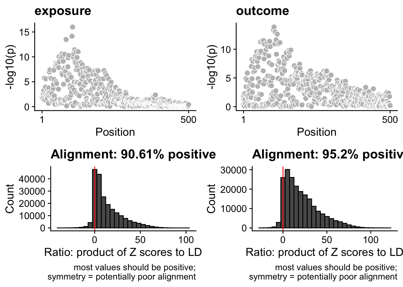
Check the causal SNP in the data
# finemap check ====
SNP_causal_exposure <- coloc::finemap.abf(dataset = data_coloc_exposure) %>%
  dplyr::filter(SNP.PP == max(SNP.PP)) %>%
  dplyr::select(snp, SNP.PP)
SNP_causal_exposure
snp SNP.PP
1 s105 0.9558118SNP_causal_outcome <- coloc::finemap.abf(dataset = data_coloc_outcome) %>%
dplyr::filter(SNP.PP == max(SNP.PP)) %>%
dplyr::select(snp, SNP.PP)
SNP_causal_outcome snp SNP.PP
1 s105 0.5922814Perform coloc across all sets of priors.
# coloc.abf ====
coloc_results <- lapply(priors, function(params) {
  coloc::coloc.abf(
    dataset1 = data_coloc_exposure,
    dataset2 = data_coloc_outcome,
    p1 = params$p1,
    p2 = params$p2,
    p12 = params$p12
  )
})
PP.H0.abf PP.H1.abf PP.H2.abf PP.H3.abf PP.H4.abf
3.35e-19 7.15e-11 8.19e-12 7.47e-04 9.99e-01
[1] "PP abf for shared variant: 99.9%"
PP.H0.abf PP.H1.abf PP.H2.abf PP.H3.abf PP.H4.abf
3.33e-18 7.10e-10 8.13e-11 7.42e-03 9.93e-01
[1] "PP abf for shared variant: 99.3%"
PP.H0.abf PP.H1.abf PP.H2.abf PP.H3.abf PP.H4.abf
3.35e-18 7.15e-10 8.19e-12 7.47e-04 9.99e-01
[1] "PP abf for shared variant: 99.9%"
PP.H0.abf PP.H1.abf PP.H2.abf PP.H3.abf PP.H4.abf
3.35e-18 7.15e-11 8.19e-11 7.47e-04 9.99e-01
[1] "PP abf for shared variant: 99.9%"
PP.H0.abf PP.H1.abf PP.H2.abf PP.H3.abf PP.H4.abf
3.35e-17 7.15e-10 8.19e-11 7.47e-04 9.99e-01
[1] "PP abf for shared variant: 99.9%"Put results in a nice table; 1 row for each prior tested.
# results table ====
table_coloc <- data.frame()
# Loop through the coloc_results list
for (j in seq_along(coloc_results)) {
  results_coloc <- coloc_results[[j]]
  results <- data.frame(
    SNP = SNP,
    finemap_snp_exposure = SNP_causal_exposure$snp,
    finemap_snp_exposure_PP = SNP_causal_exposure$SNP.PP,
    finemap_snp_outcome = SNP_causal_outcome$snp,
    finemap_snp_outcome_PP = SNP_causal_outcome$SNP.PP,
    nsnps = results_coloc$summary[["nsnps"]],
    h0 = results_coloc$summary[["PP.H0.abf"]],
    h1 = results_coloc$summary[["PP.H1.abf"]],
    h2 = results_coloc$summary[["PP.H2.abf"]],
    h3 = results_coloc$summary[["PP.H3.abf"]],
    h4 = results_coloc$summary[["PP.H4.abf"]],
    prior_p1 = results_coloc$priors[["p1"]],
    prior_p2 = results_coloc$priors[["p2"]],
    prior_p12 = results_coloc$priors[["p12"]],
    priors_label = label_priors[j]
  )
  # Bind the current results to the accumulated table
  table_coloc <- bind_rows(table_coloc, results)
}
Run sensitivity analysis
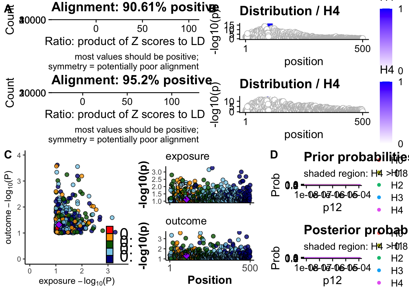
# sensitivity  ====
plot <- functions::coloc_sensitivity(
  obj = coloc_results[[1]],
  rule = "H4 > 0.8", npoints = 100, row = 1, suppress_messages = TRUE,
  trait1_title = "exposure", trait2_title = "outcome",
  dataset1 = NULL, dataset2 = NULL,
  data_check_trait1 = data_coloc_exposure, data_check_trait2 = data_coloc_outcome
)
ggsave("plot-sensitivity.png", plot, width = 4000, height = 4000, units = "px")
Warning: ggrepel: 1 unlabeled data points (too many overlaps). Consider
increasing max.overlapsCheck results and sensitivity analysis
knitr::kable(table_coloc)| SNP | finemap_snp_exposure | finemap_snp_exposure_PP | finemap_snp_outcome | finemap_snp_outcome_PP | nsnps | h0 | h1 | h2 | h3 | h4 | prior_p1 | prior_p2 | prior_p12 | priors_label |
|---|---|---|---|---|---|---|---|---|---|---|---|---|---|---|
| s105 | s105 | 0.9558118 | s105 | 0.5922814 | 500 | 0 | 0 | 0 | 0.0007475 | 0.9992525 | 1e-04 | 1e-04 | 1e-05 | p1=1e-4;p2=1e-4;p12=1e-5 |
| s105 | s105 | 0.9558118 | s105 | 0.5922814 | 500 | 0 | 0 | 0 | 0.0074249 | 0.9925751 | 1e-04 | 1e-04 | 1e-06 | p1=1e-4;p2=1e-4;p12=1e-6 |
| s105 | s105 | 0.9558118 | s105 | 0.5922814 | 500 | 0 | 0 | 0 | 0.0007475 | 0.9992525 | 1e-04 | 1e-05 | 1e-06 | p1=1e-4;p2=1e-5;p12=1e-6 |
| s105 | s105 | 0.9558118 | s105 | 0.5922814 | 500 | 0 | 0 | 0 | 0.0007475 | 0.9992525 | 1e-05 | 1e-04 | 1e-06 | p1=1e-5;p2=1e-4;p12=1e-6 |
| s105 | s105 | 0.9558118 | s105 | 0.5922814 | 500 | 0 | 0 | 0 | 0.0007475 | 0.9992525 | 1e-05 | 1e-05 | 1e-07 | p1=1e-5;p2=1e-5;p12=1e-7 |
plot