Mendelian Randomization Workflow

library(functions)
library(dplyr)
library(tidyr)
library(TwoSampleMR)

End-to-End MR Analysis

This vignette demonstrates a complete workflow for Mendelian Randomization analysis.

1. Data Preparation

We’ll start by creating mock GWAS data for both an exposure and an outcome.

set.seed(123)

# Mock exposure data
exp_raw <- data.frame(
  SNP = paste0("rs", 1:30),
  beta = rnorm(30, 0.5, 0.1),
  se = runif(30, 0.01, 0.05),
  effect_allele = "A",
  other_allele = "G",
  eaf = runif(30, 0.1, 0.9),
  pval = 10^(-runif(30, 5, 10)),
  samplesize = 10000,
  phenotype = "Exposure Trait"
)

# Mock outcome data
out_raw <- data.frame(
  SNP = paste0("rs", 1:100),
  beta = rnorm(100, 0, 0.1),
  se = runif(100, 0.02, 0.06),
  effect_allele = "A",
  other_allele = "G",
  eaf = runif(100, 0.1, 0.9),
  pval = runif(100),
  phenotype = "Outcome Trait"
)

exp_dat <- format_data(exp_raw, type = "exposure")
out_dat <- format_data(out_raw, type = "outcome")

2. Instrument Strength

The functions package provides utilities to calculate instrument strength ( $R^2$ and $F$ -statistic).

Variance Explained ( $R^2$ )

Calculate the proportion of variance explained by the instruments using calculate_r2.

exp_dat <- calculate_r2(exp_dat)
head(exp_dat |> select(SNP, beta.exposure, r2))
#>   SNP beta.exposure         r2
#> 1 rs1     0.4439524 0.01449638
#> 2 rs2     0.4769823 0.10680549
#> 3 rs3     0.6558708 0.06269876
#> 4 rs4     0.5070508 0.05521028
#> 5 rs5     0.5129288 0.01429991
#> 6 rs6     0.6715065 0.05460598

F-statistic from $R^2$

The F-statistic can be calculated based on $R^2$ , sample size ( $N$ ), and number of instruments ( $k$ ).

# grouping_column determines how to aggregate SNPs (e.g., by phenotype/exposure)
f_stat_res <- calculate_fstat_from_r2(exp_dat, grouping_column = exposure)
unique(f_stat_res |> select(exposure, mean_fstat_from_r2))
#> # A tibble: 1 × 2
#>   exposure mean_fstat_from_r2
#>   <chr>                 <dbl>
#> 1 exposure               16.1

F-statistic from Beta and SE

Alternatively, calculate the F-statistic directly from effect sizes and standard errors.

exp_dat <- calculate_fstat_from_beta_se(exp_dat)
head(exp_dat |> select(SNP, fstat_from_b_se, mean_f_stats))
#>   SNP fstat_from_b_se mean_f_stats
#> 1 rs1        147.0962     484.5334
#> 2 rs2       1195.7696     484.5334
#> 3 rs3        668.9286     484.5334
#> 4 rs4        584.3657     484.5334
#> 5 rs5        145.0737     484.5334
#> 6 rs6        577.6002     484.5334

3. Harmonization and Analysis

harmonized <- TwoSampleMR::harmonise_data(exp_dat, out_dat, action = 2)
res <- TwoSampleMR::mr(harmonized)

4. Custom Visualization

The functions package provides enhanced versions of standard MR plots. Key differences from the TwoSampleMR package include: - Improved Labelling: Plots automatically include trait names in titles and axes. - SNP Ordering: Forest and Leave-one-out plots order SNPs by effect size for better clarity. - Styling: Uses custom color palettes and unified themes suitable for publication.

Scatter Plot

Enhances the standard scatter plot by adding trait labels and enforcing positive exposure effects (flipping signs for consistency).

# Returns a list of plots
plots <- mr_scatter_plot(res, harmonized)
plots[[1]]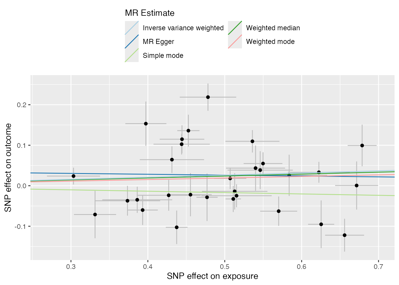

Forest Plot

Standardizes method names (e.g., “IVW”) and separates individual SNP effects from pooled estimates with a gap.

singlesnp_res <- TwoSampleMR::mr_singlesnp(harmonized)
plots <- mr_forest_plot(singlesnp_res)
plots[[1]]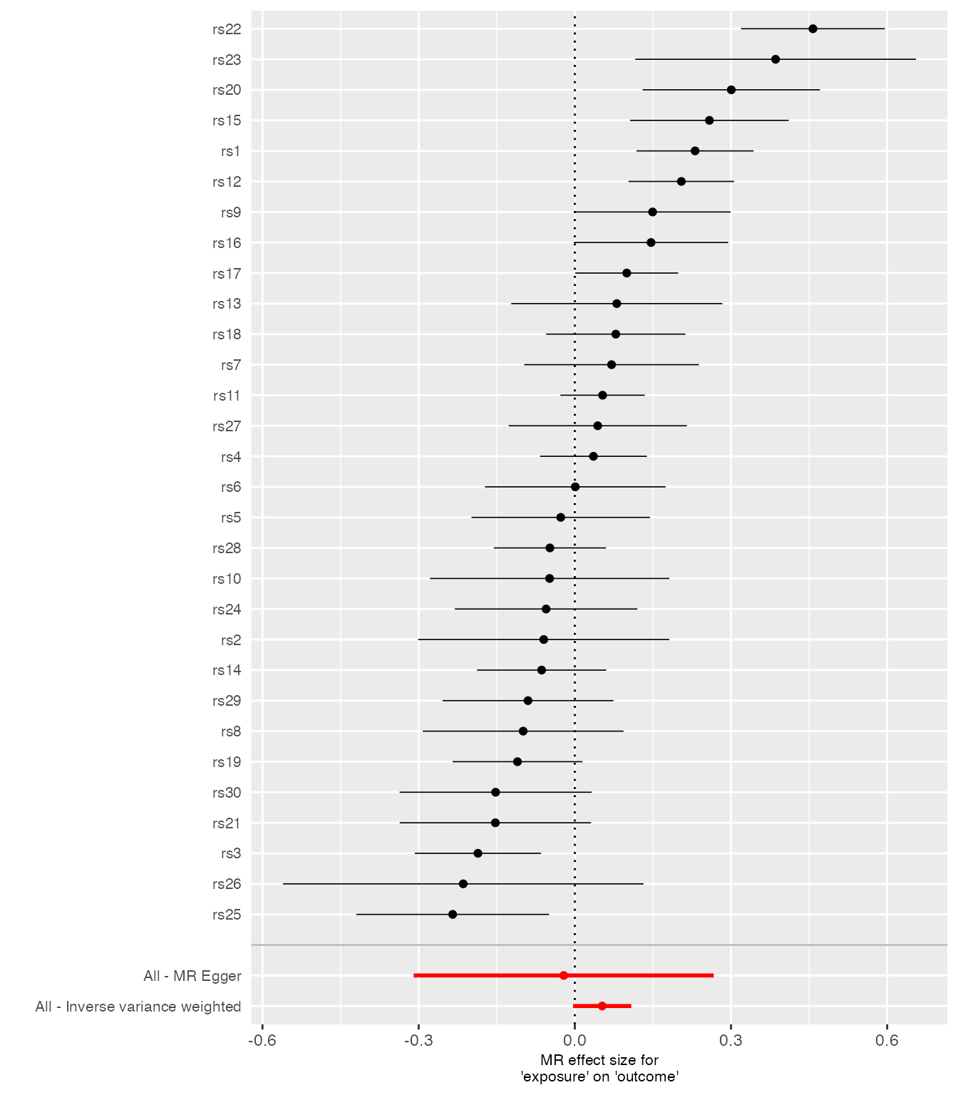

Funnel Plot

Uses a specific high-contrast color palette and clear title mapping.

plots <- mr_funnel_plot(singlesnp_res)
plots[[1]]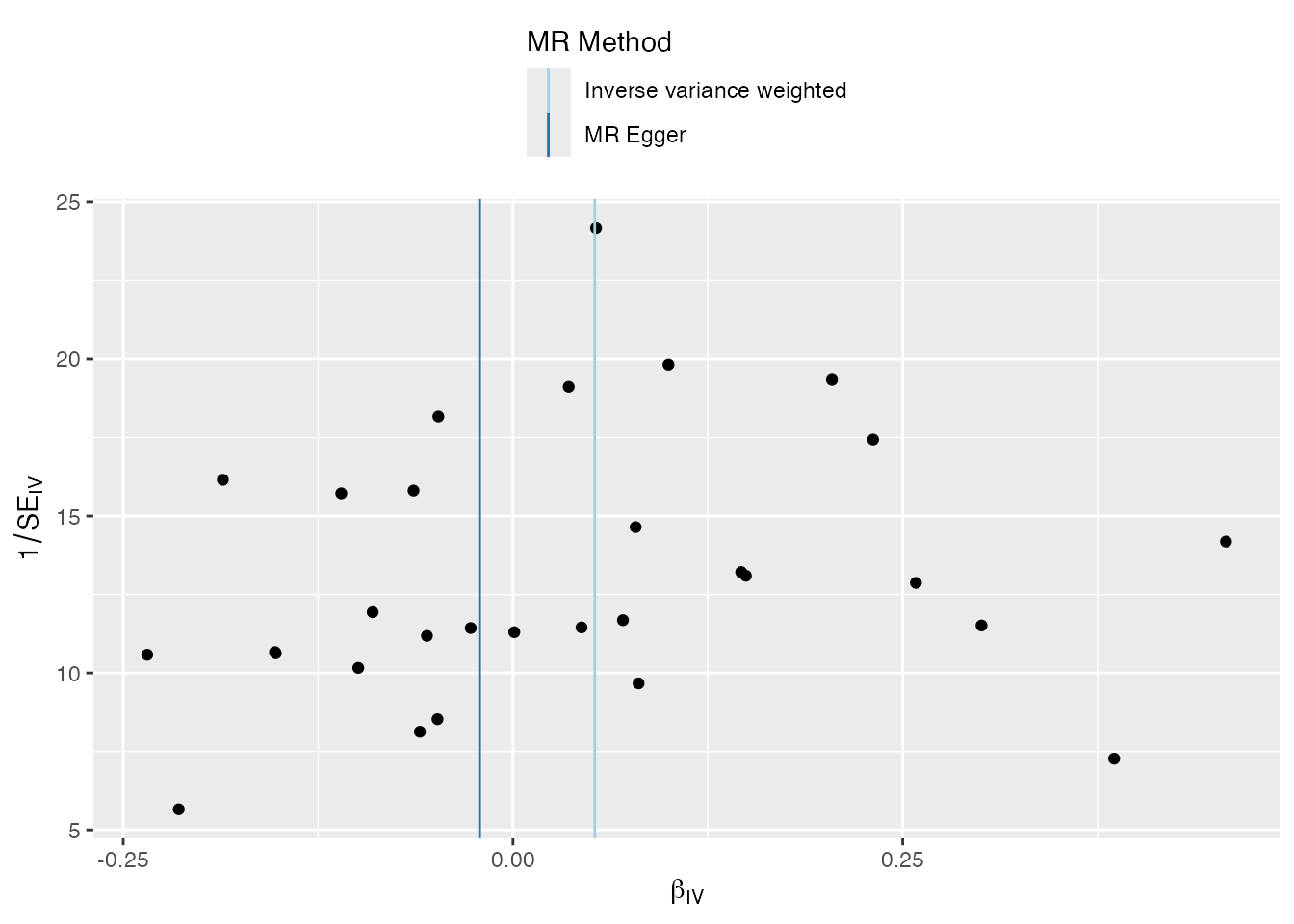

Leave-one-out Plot

Visually identifies SNPs driving the MR result by ordering entries.

loo_res <- TwoSampleMR::mr_leaveoneout(harmonized)
plots <- mr_leaveoneout_plot(loo_res)
plots[[1]]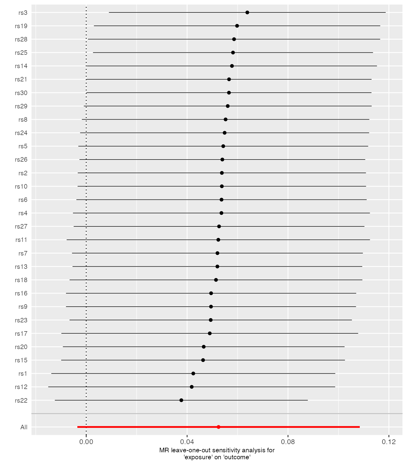

Density Plot

Weighted density estimation of per-SNP effects to visualize the distribution of estimates.

plots <- mr_density_plot(singlesnp_res, res)
plots[[1]]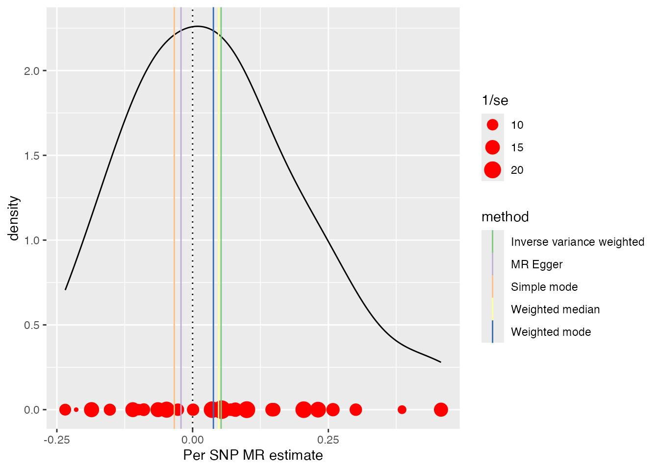

5. Directional Consistency

directional_consistency checks whether the effect estimate remains in the same direction across different MR results.

# Create 4 results with positive effects for demonstration
set.seed(42)
res1 <- res |> mutate(id.exposure = "Study A", b = abs(b))
res2 <- res |> mutate(id.exposure = "Study B", b = abs(b) * 1.1)
res3 <- res |> mutate(id.exposure = "Study C", b = abs(b) * 0.9)
res4 <- res |> mutate(id.exposure = "Study D", b = abs(b) * 1.5)

# Pivot to wide format as required by the function
wide_res <- bind_rows(res1, res2, res3, res4) |>
  select(method, id.exposure, b) |>
  pivot_wider(names_from = id.exposure, values_from = b)

# Check consistency
consistency <- directional_consistency(as.data.frame(wide_res))
consistency
#>                           direction direction_group
#> MR Egger                          1        positive
#> Weighted median                   1        positive
#> Inverse variance weighted         1        positive
#> Simple mode                       1        positive
#> Weighted mode                     1        positive