Colocalisation Analysis

library(functions)
library(coloc)
library(dplyr)
library(ggplot2)
library(cowplot)

Introduction to Colocalisation

Colocalisation analysis tests whether two traits share a common causal variant at a genomic locus. This is particularly useful in genetics to determine if:

A GWAS signal and an eQTL signal are driven by the same variant
Two different traits share the same genetic architecture at a locus
A disease risk variant operates through a specific molecular mechanism

The coloc package implements Bayesian methods to evaluate five hypotheses:

H0: No association with either trait
H1: Association with trait 1 only
H2: Association with trait 2 only
H3: Association with both traits, but different causal variants
H4: Association with both traits, shared causal variant (colocalisation)

Colocalisation Data Structure

The coloc package requires data in a specific list format. Each dataset must contain:

Required Components

beta: Effect sizes for each SNP (numeric vector)
varbeta: Variance of effect sizes (numeric vector)
snp: SNP identifiers (character vector)
position: Genomic positions (numeric vector)
type: Either "quant" (quantitative trait) or "cc" (case-control)
MAF: Minor allele frequency (numeric vector, optional but recommended)
N: Sample size (single number or vector)
LD: Linkage disequilibrium matrix (matrix with SNP names as dimnames)

Optional Components

sdY: Standard deviation of the phenotype (for quantitative traits)
s: Proportion of samples that are cases (for case-control studies)
pval: P-values (optional, for visualization)

Example Data Preparation

We’ll use the test data from the coloc package to demonstrate the workflow:

# Load test data from coloc package
data(coloc_test_data)

# Prepare exposure dataset (quantitative trait, e.g., gene expression)
data_coloc_exposure <- coloc_test_data$D1[c("beta", "varbeta", "snp", "position", "type", "sdY", "LD", "MAF")]
data_coloc_exposure$N <- 10000
data_coloc_exposure$chr <- 1
data_coloc_exposure$pval <- runif(n = length(data_coloc_exposure$snp), min = 5e-200, max = 0.1)

# Prepare outcome dataset (case-control trait, e.g., disease)
data_coloc_outcome <- coloc_test_data$D2[c("beta", "varbeta", "snp", "position", "LD", "MAF")]
data_coloc_outcome$type <- "cc"
data_coloc_outcome$N <- 10000
data_coloc_outcome$chr <- 1
data_coloc_outcome$pval <- runif(n = length(data_coloc_outcome$snp), min = 5e-200, max = 0.1)

# Verify structure
str(data_coloc_exposure, max.level = 1)
#> List of 11
#>  $ beta    : num [1:500] 0.337 0.211 0.257 0.267 0.247 ...
#>  $ varbeta : num [1:500] 0.01634 0.00532 0.00748 0.01339 0.00664 ...
#>  $ snp     : chr [1:500] "s1" "s2" "s3" "s4" ...
#>  $ position: int [1:500] 1 2 3 4 5 6 7 8 9 10 ...
#>  $ type    : chr "quant"
#>  $ sdY     : num 1.1
#>  $ LD      : num [1:500, 1:500] 1 0.365 0.54 0.851 0.463 ...
#>   ..- attr(*, "dimnames")=List of 2
#>  $ MAF     : num [1:500] 0.031 0.166 0.0925 0.0405 0.118 ...
#>  $ N       : num 10000
#>  $ chr     : num 1
#>  $ pval    : num [1:500] 0.00808 0.08343 0.06008 0.01572 0.00074 ...
str(data_coloc_outcome, max.level = 1)
#> List of 10
#>  $ beta    : num [1:500] 0.0926 0.1661 0.1519 0.0342 0.214 ...
#>  $ varbeta : num [1:500] 0.01403 0.00467 0.00649 0.01151 0.00593 ...
#>  $ snp     : chr [1:500] "s1" "s2" "s3" "s4" ...
#>  $ position: int [1:500] 1 2 3 4 5 6 7 8 9 10 ...
#>  $ LD      : num [1:500, 1:500] 1 0.365 0.54 0.851 0.463 ...
#>   ..- attr(*, "dimnames")=List of 2
#>  $ MAF     : num [1:500] 0.031 0.166 0.0925 0.0405 0.118 ...
#>  $ type    : chr "cc"
#>  $ N       : num 10000
#>  $ chr     : num 1
#>  $ pval    : num [1:500] 0.02032 0.00683 0.03073 0.09931 0.01163 ...

Data Quality Checks

Before running colocalisation analysis, always verify your data:

# Check datasets using coloc's built-in validation
coloc::check_dataset(d = data_coloc_exposure, suffix = 1, warn.minp = 5e-8)
#> NULL
coloc::check_dataset(d = data_coloc_outcome, suffix = 2, warn.minp = 5e-8)
#> NULL

Checking Data Alignment

The coloc_check_alignment() function verifies that effect alleles are correctly aligned between datasets by comparing Z-score products to LD patterns.

# Create alignment plots for both datasets
plot_grid(
    coloc_check_alignment(D = data_coloc_exposure),
    coloc_check_alignment(D = data_coloc_outcome),
    ncol = 2,
    labels = c("Exposure", "Outcome")
)

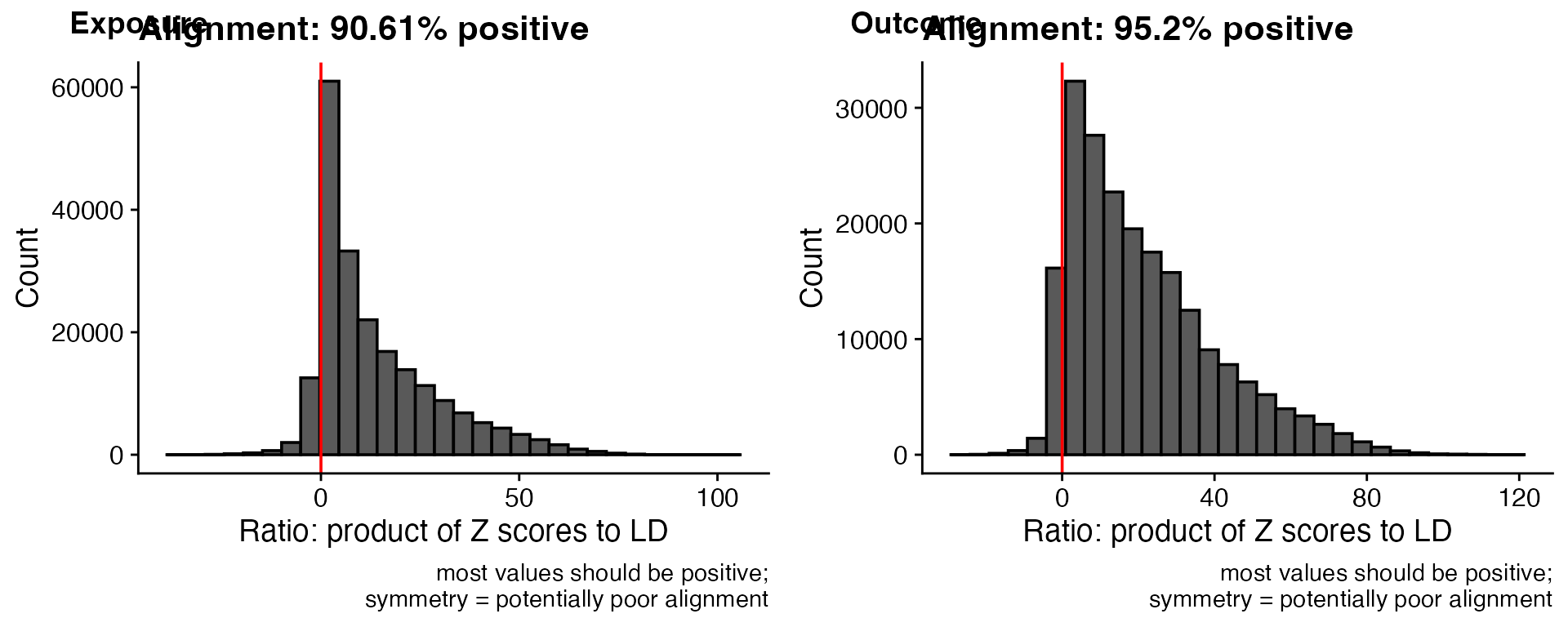
Interpretation: - Most values positive: Good alignment (effect alleles correctly coded) - Symmetric distribution: Poor alignment (potential strand/allele flips) - Aim for >90% positive values for reliable colocalisation results

# Get numeric alignment scores
alignment_exposure <- coloc_check_alignment(data_coloc_exposure, do_plot = FALSE)
alignment_outcome <- coloc_check_alignment(data_coloc_outcome, do_plot = FALSE)

cat("Exposure alignment:", round(alignment_exposure * 100, 2), "% positive\n")
#> Exposure alignment: 90.61 % positive
cat("Outcome alignment:", round(alignment_outcome * 100, 2), "% positive\n")
#> Outcome alignment: 95.2 % positive

Visualizing Datasets

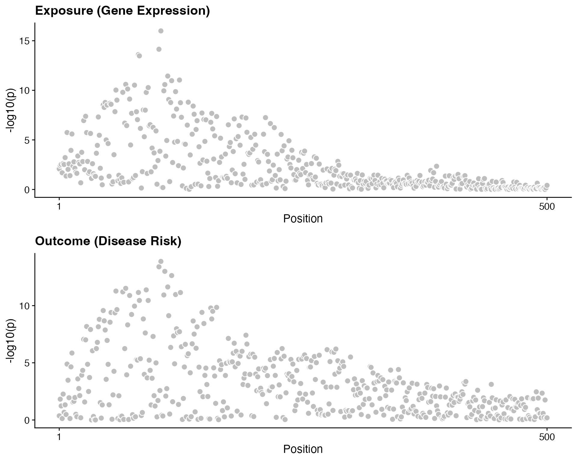
Before colocalisation, visualize the association patterns:

plot_grid(
    coloc_plot_dataset(d = data_coloc_exposure, label = "Exposure (Gene Expression)"),
    coloc_plot_dataset(d = data_coloc_outcome, label = "Outcome (Disease Risk)"),
    ncol = 1
)

Fine-mapping to Identify Causal Variants

Use Bayesian fine-mapping to identify the most likely causal variant in each dataset:

# Fine-map exposure
SNP_causal_exposure <- coloc::finemap.abf(dataset = data_coloc_exposure) |>
    dplyr::filter(SNP.PP == max(SNP.PP)) |>
    dplyr::select(snp, SNP.PP)

# Fine-map outcome
SNP_causal_outcome <- coloc::finemap.abf(dataset = data_coloc_outcome) |>
    dplyr::filter(SNP.PP == max(SNP.PP)) |>
    dplyr::select(snp, SNP.PP)

cat(
    "Most likely causal SNP in exposure:", SNP_causal_exposure$snp,
    "(PP =", round(SNP_causal_exposure$SNP.PP, 3), ")\n"
)
#> Most likely causal SNP in exposure: s105 (PP = 0.956 )
cat(
    "Most likely causal SNP in outcome:", SNP_causal_outcome$snp,
    "(PP =", round(SNP_causal_outcome$SNP.PP, 3), ")\n"
)
#> Most likely causal SNP in outcome: s105 (PP = 0.592 )

Running Colocalisation Analysis

Single Analysis with Default Priors

# Run coloc with default priors
coloc_result <- coloc::coloc.abf(
    dataset1 = data_coloc_exposure,
    dataset2 = data_coloc_outcome
)
#> PP.H0.abf PP.H1.abf PP.H2.abf PP.H3.abf PP.H4.abf 
#>  3.35e-19  7.15e-11  8.19e-12  7.47e-04  9.99e-01 
#> [1] "PP abf for shared variant: 99.9%"

# View summary
print(coloc_result$summary)
#>        nsnps    PP.H0.abf    PP.H1.abf    PP.H2.abf    PP.H3.abf    PP.H4.abf 
#> 5.000000e+02 3.349762e-19 7.145521e-11 8.188561e-12 7.474844e-04 9.992525e-01

Interpreting Results

The posterior probabilities indicate support for each hypothesis:

PP.H0.abf: No association
PP.H1.abf: Exposure only
PP.H2.abf: Outcome only
PP.H3.abf: Both traits, different variants
PP.H4.abf: Colocalisation (shared variant)

Decision rules: - PP.H4 > 0.8: Strong evidence for colocalisation - PP.H3 > 0.8: Strong evidence for distinct causal variants - PP.H4 + PP.H3 < 0.8: Inconclusive

Testing Multiple Prior Scenarios

Colocalisation results can be sensitive to prior assumptions. Test multiple scenarios:

# Define different prior scenarios
priors <- list(
    list(p1 = 1e-4, p2 = 1e-4, p12 = 1e-5),
    list(p1 = 1e-4, p2 = 1e-4, p12 = 1e-6),
    list(p1 = 1e-4, p2 = 1e-5, p12 = 1e-6),
    list(p1 = 1e-5, p2 = 1e-4, p12 = 1e-6),
    list(p1 = 1e-5, p2 = 1e-5, p12 = 1e-7)
)

label_priors <- c(
    "p1=1e-4; p2=1e-4; p12=1e-5",
    "p1=1e-4; p2=1e-4; p12=1e-6",
    "p1=1e-4; p2=1e-5; p12=1e-6",
    "p1=1e-5; p2=1e-4; p12=1e-6",
    "p1=1e-5; p2=1e-5; p12=1e-7"
)

# Run coloc for each prior scenario
coloc_results <- lapply(priors, function(params) {
    coloc::coloc.abf(
        dataset1 = data_coloc_exposure,
        dataset2 = data_coloc_outcome,
        p1 = params$p1,
        p2 = params$p2,
        p12 = params$p12
    )
})
#> PP.H0.abf PP.H1.abf PP.H2.abf PP.H3.abf PP.H4.abf 
#>  3.35e-19  7.15e-11  8.19e-12  7.47e-04  9.99e-01 
#> [1] "PP abf for shared variant: 99.9%"
#> PP.H0.abf PP.H1.abf PP.H2.abf PP.H3.abf PP.H4.abf 
#>  3.33e-18  7.10e-10  8.13e-11  7.42e-03  9.93e-01 
#> [1] "PP abf for shared variant: 99.3%"
#> PP.H0.abf PP.H1.abf PP.H2.abf PP.H3.abf PP.H4.abf 
#>  3.35e-18  7.15e-10  8.19e-12  7.47e-04  9.99e-01 
#> [1] "PP abf for shared variant: 99.9%"
#> PP.H0.abf PP.H1.abf PP.H2.abf PP.H3.abf PP.H4.abf 
#>  3.35e-18  7.15e-11  8.19e-11  7.47e-04  9.99e-01 
#> [1] "PP abf for shared variant: 99.9%"
#> PP.H0.abf PP.H1.abf PP.H2.abf PP.H3.abf PP.H4.abf 
#>  3.35e-17  7.15e-10  8.19e-11  7.47e-04  9.99e-01 
#> [1] "PP abf for shared variant: 99.9%"

# Create results table
table_coloc <- data.frame()
for (j in seq_along(coloc_results)) {
    results_coloc <- coloc_results[[j]]
    results <- data.frame(
        scenario = label_priors[j],
        nsnps = results_coloc$summary[["nsnps"]],
        PP.H0 = results_coloc$summary[["PP.H0.abf"]],
        PP.H1 = results_coloc$summary[["PP.H1.abf"]],
        PP.H2 = results_coloc$summary[["PP.H2.abf"]],
        PP.H3 = results_coloc$summary[["PP.H3.abf"]],
        PP.H4 = results_coloc$summary[["PP.H4.abf"]],
        p1 = results_coloc$priors[["p1"]],
        p2 = results_coloc$priors[["p2"]],
        p12 = results_coloc$priors[["p12"]]
    )
    table_coloc <- dplyr::bind_rows(table_coloc, results)
}

# Display results
print(table_coloc)
#>                     scenario nsnps        PP.H0        PP.H1        PP.H2
#> 1 p1=1e-4; p2=1e-4; p12=1e-5   500 3.349762e-19 7.145521e-11 8.188561e-12
#> 2 p1=1e-4; p2=1e-4; p12=1e-6   500 3.327378e-18 7.097771e-10 8.133842e-11
#> 3 p1=1e-4; p2=1e-5; p12=1e-6   500 3.349762e-18 7.145521e-10 8.188561e-12
#> 4 p1=1e-5; p2=1e-4; p12=1e-6   500 3.349762e-18 7.145521e-11 8.188561e-11
#> 5 p1=1e-5; p2=1e-5; p12=1e-7   500 3.349762e-17 7.145521e-10 8.188561e-11
#>          PP.H3     PP.H4    p1    p2   p12
#> 1 0.0007474844 0.9992525 1e-04 1e-04 1e-05
#> 2 0.0074248936 0.9925751 1e-04 1e-04 1e-06
#> 3 0.0007474844 0.9992525 1e-04 1e-05 1e-06
#> 4 0.0007474844 0.9992525 1e-05 1e-04 1e-06
#> 5 0.0007474844 0.9992525 1e-05 1e-05 1e-07

Comprehensive Sensitivity Analysis

The coloc_sensitivity() function provides a complete sensitivity analysis with visualizations:

# Run comprehensive sensitivity analysis
sensitivity_plot <- coloc_sensitivity(
    obj = coloc_results[[1]],
    rule = "H4 > 0.8",
    npoints = 100,
    row = 1,
    suppress_messages = TRUE,
    trait1_title = "Gene Expression",
    trait2_title = "Disease Risk",
    dataset1 = NULL,
    dataset2 = NULL,
    data_check_trait1 = data_coloc_exposure,
    data_check_trait2 = data_coloc_outcome
)

# Display the sensitivity plot
sensitivity_plot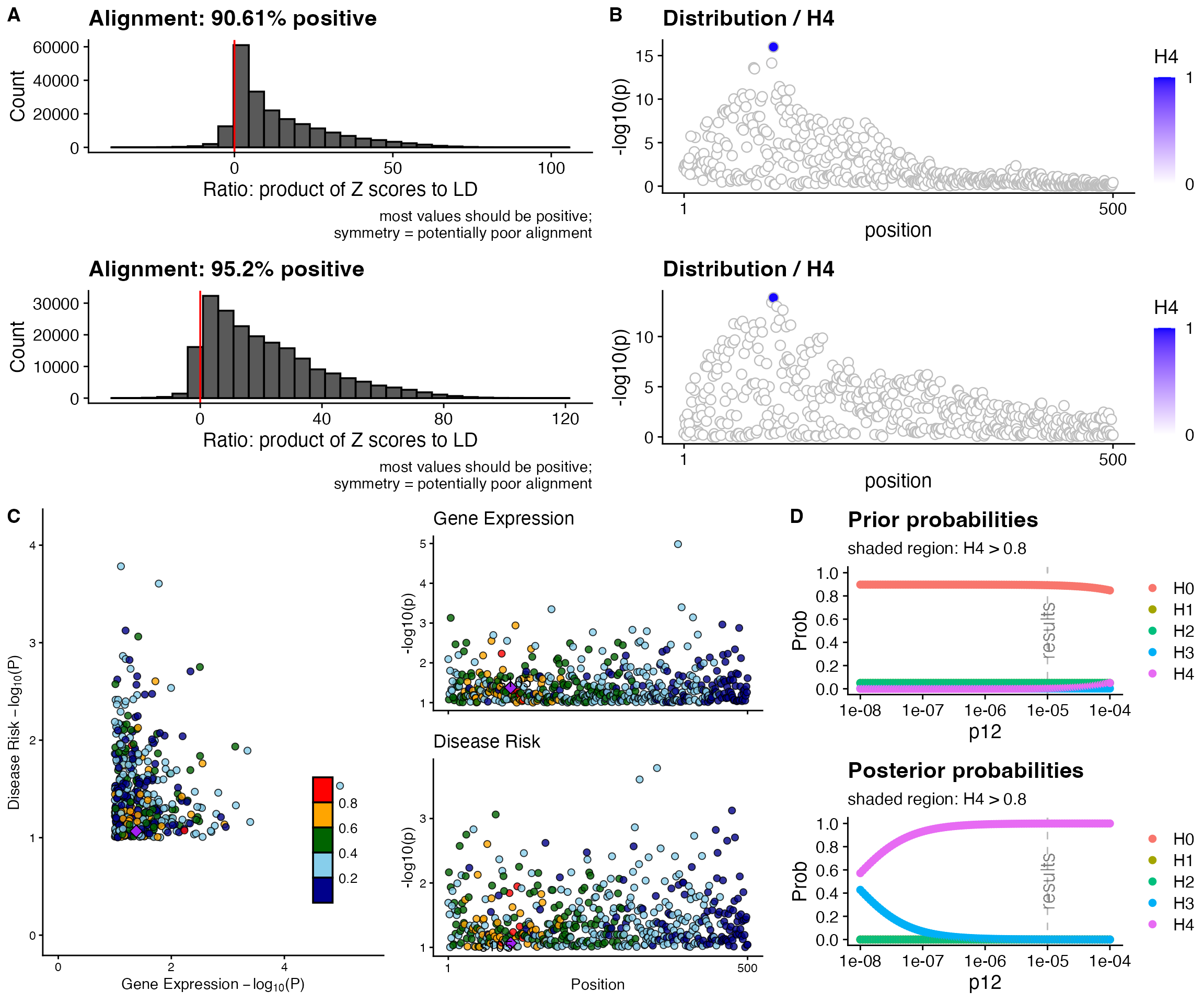

Understanding the Sensitivity Plot

The comprehensive sensitivity plot contains four panels:

Panel A: Alignment Checks - Histograms showing the ratio of Z-score products to LD - Should be predominantly positive (>90%) - Symmetric distributions indicate alignment problems

Panel B: Manhattan Plots - Regional association patterns for both traits - Points colored by SNP-level PP.H4 - Blue indicates higher posterior probability of being the shared causal variant

Panel C: LocusCompare - Scatter plot comparing -log10(p-values) between traits - Points colored by LD with the lead SNP - Helps visualize if the same variant drives both signals

Panel D: Prior/Posterior Sensitivity - Top plot: How prior probabilities change with p12 - Bottom plot: How posterior probabilities change with p12 - Green shaded region: Range of p12 values where PP.H4 > 0.8

Interpreting the green region: - Wide green region: Robust result, insensitive to prior choice ✓ - Narrow green region: Moderately sensitive, interpret with caution - No green region: Weak evidence, highly sensitive to priors

Best Practices

1. Always Check Alignment First

# Poor alignment invalidates results
if (alignment_exposure < 0.7 || alignment_outcome < 0.7) {
    warning("Poor alignment detected! Review allele coding before proceeding.")
}

2. Use Appropriate Priors

# For well-powered GWAS with many SNPs
stringent_priors <- list(p1 = 1e-5, p2 = 1e-5, p12 = 1e-7)

# For candidate gene studies with fewer SNPs
relaxed_priors <- list(p1 = 1e-4, p2 = 1e-4, p12 = 1e-5)

3. Consider the Biological Context

eQTL + GWAS: Expect many eQTLs (higher p1), fewer GWAS hits (lower p2)
Two GWAS traits: Use similar p1 and p2 values
Shared mechanisms: Higher p12 may be appropriate

4. Report Sensitivity

Always report how robust your conclusions are to prior assumptions:

# Check if PP.H4 > 0.8 across all scenarios
robust <- all(table_coloc$PP.H4 > 0.8)
cat("Result robust across all prior scenarios:", robust, "\n")
#> Result robust across all prior scenarios: TRUE

Common Issues and Solutions

Issue 1: Low PP.H4 Across All Scenarios

Possible causes: - No true association in one or both traits - Different causal variants (check PP.H3) - Insufficient LD coverage

Solution: - Verify both traits show strong association - Ensure good LD coverage around the signal - Consider expanding the genomic window

Issue 2: Symmetric Alignment Distribution

Possible causes: - Strand flips between datasets - Incorrect effect allele coding - Mixed reference panels

Solution: - Harmonize to the same reference strand - Verify effect allele definitions - Use consistent reference panels

Issue 3: Highly Sensitive to Priors

Possible causes: - Weak associations - Insufficient sample size - Ambiguous genetic architecture

Solution: - Seek replication in independent datasets - Increase sample size if possible - Report uncertainty clearly

Summary

The functions package enhances colocalisation analysis with:

coloc_check_alignment(): Verify data quality before analysis
coloc_sensitivity(): Comprehensive sensitivity analysis with multi-panel visualizations
coloc_plot_dataset(): Visualize regional association patterns
coloc_manh.plot(): Manhattan plots colored by PP.H4
coloc_prior.snp2hyp(): Convert SNP-level priors to hypothesis priors
coloc_prior.adjust(): Adjust posterior probabilities for different priors

Key Takeaways

Always check alignment before interpreting results
Test multiple prior scenarios to assess robustness
Use the sensitivity plot to understand prior dependence
Report PP.H3 and PP.H4 together for complete interpretation
Seek replication when results are sensitive to priors